4 Guide
ADViSELipidomics has a graphical user interface (GUI) implemented using the shiny and golem R packages. It has five main sections: Home, Data Import & Preprocessing, SumExp Visualization, Exploratory Analysis, and Statistical Analysis. Each section is accessible from a sidemenu on the left.
4.1 Home section
The Home section includes general information about ADViSELipidomics as the citation, the link to the GitHub page, and the link to this manual. From the “Start!” button, it is possible to go to the following section where the user can upload the lipidomic data.
4.2 Data Import & Preprocessing
This section allows to import and process lipidomic data from various sources. When you open this section for the first time after launch, a message box appears and asks you to write your name and your company. This information will be stored in the final output of ADViSELipidomics. By default, if you click on “Run” the User will be “Name” and the Company will be “Company”. The picture below shows the Data Import & Preprocessing section (with the different parts enlightened with red rectangles).
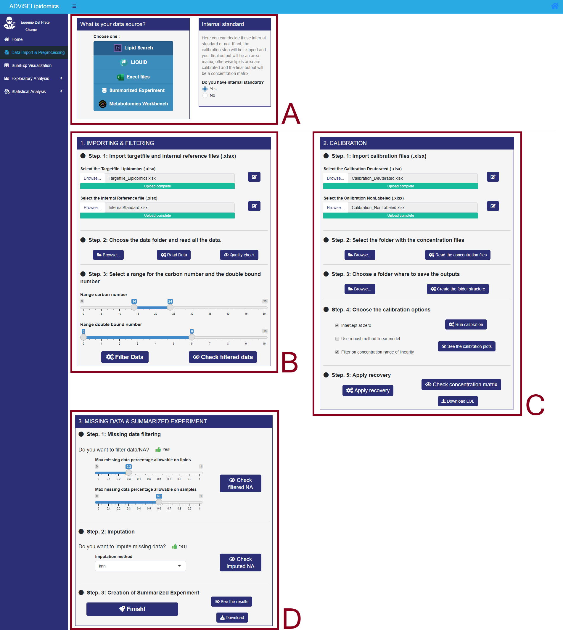
- Rectangle A allows the user to choose between LipidSearch, LIQUID, Excel files, Summarized Experiment, and Metabolomics Workbench. Moreover, it is also possible to select between experiments with or without internal standards (this option is available only for LipidSearch import).
- Rectangle B shows three different steps for Importing & Filtering: importing data, storing, and reading data, filtering data.
- Rectangle C shows five additional steps for Calibration: importing calibration files, storing calibration files, selecting the folder for the results, selecting calibration options, application of recovery.
- Rectangle D shows two different steps for Filtering and Missing Data imputation and creating the SummarizedExperiment object. Note that the layout of the Data Import & Preprocessing section and the required files depends on the type of input data format choosen by the user. Go to Chapter 3 if you need help gathering all the required files.
Since the option LipidSearch output with Internal Standard (IS) has the largest number of required files and steps, here we provide a complete guide for this case. Anyway, this guide applies also to LipidSearch without IS and to LIQUID: in these cases, the only difference is that there isn’t the CALIBRATION module (Section 4.2.2).
4.2.1 LipidSearch (IS) EXAMPLE - IMPORTING & FILTERING module
The first module is the IMPORTING & FILTERING module, where the user can upload the Target File, the Internal Reference File, and the Data files from LipidSearch.
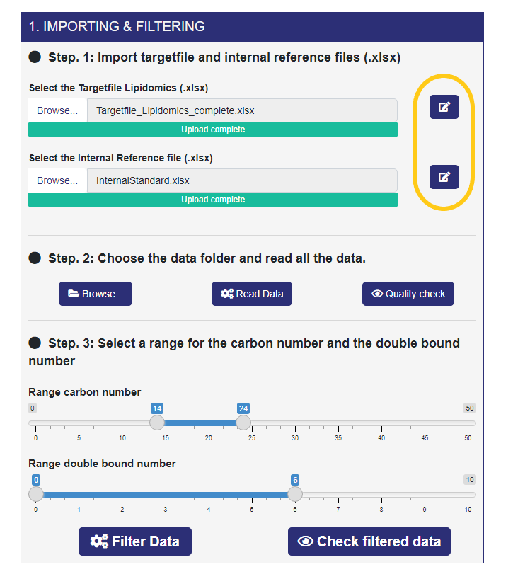
- Step 1. The first files that you must import are the Target File and the Internal Reference File (Rectangle A, steps 1 and 2). Next to each of them there is a button (yellow squared rectangle) that allows you to edit the Excel files. You can filter the rows by one or more conditions, select only the needed columns, and download the edited data. To apply the editing, you have to enable the button next to the download button and click on the “Done” button (right-top corner). Anyway, a help button guides you through the editing options.
- Step 2. Here, you choose the folder containing the data files coming from LipidSearch (only the data files related to the samples and NOT to the IS). After selecting the folder, click on the “Read Data” button, and ADViSELipidomics will start reading all the data files. A progress bar shows the percentage of completion. When the reading process is completed, you can perform a quality check on the area of each sample by clicking the “Quality check” button.
- Step 3. Finally, here you can filter non-informative lipids based on retention time in the range, number of carbon atoms in the range, even number of carbon atoms, number of double bonds in the range, duplicated lipids. The two sliders allows you to choose the range for the carbon number and the double bound number. The other filters come from the Internal Reference File. If there are duplicated lipids (same m/z values for lipid peaks), ADViSELipidomics takes only the lipids with the maximum peak area. The “Filter Data” button starts this process. In the end, you can check the filtered data for each sample.
4.2.2 LipidSearch (IS) EXAMPLE - CALIBRATION module
If the previous module is completed, the CALIBRATION module appears next to it. The Calibration module creates the calibration curves and the calibration matrix. It uses the Internal Lipid Standards reported in the Internal Reference file, and the correspondence between the Concentration Files and the lipid classes declared in the Calibration File. This module extracts the relationships between peaks area and concentration values for each internal lipid standard, constructing the calibration curves with a linear model and plotting them. The linear regression model can be classical or robust, with zero or non-zero intercept. Finally, the calibration matrix resumes all the points from the calibration curves. After the calibration process, ADViSELipidomics stores slope and intercept values for the recovery module. As already stated, this module appears only if you are using LipidSearch output with Internal Standard (and you clicked on “Yes” in the radiobutton that asks you “Do you have internal standards?”). In this module, you need two Calibration Files (.xlsx, see Section 3.4) and the Concentration files coming from LipidSearch related to the internal standard (.txt, see Section 3.1).
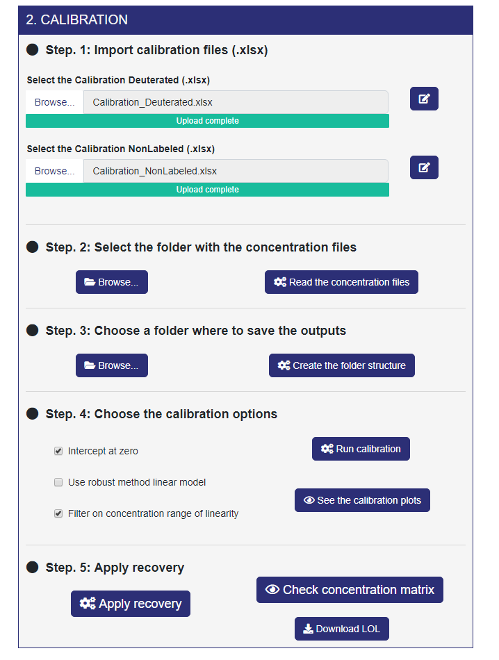
- Step. 1 Here, you can upload the Calibration Files (.xlsx) for both Deuterated and Nonlabeled. This step is remarkably similar to Step 1 of the IMPORTING & FILTERING module. You can find further information about these files in Section 3.4.
- Step. 2 Select the folder containing the Concentration files coming from LipidSearch and click on “Read the concentration files”. Also, this step is very similar to step 2 of the previous module.
- Step. 3 Here, you can select the folder where saving the output from LipidSearch. ADViSELipidomics creates for you the folder structure.
- Step. 4 In this step you can choose some calibration options and visualize the calibration plot for each standard.
- Step. 5. Finally, you can apply the recovery percentage to the concentration values for each lipid, considering the Internal Lipid Standards as lipid class reference. This normalization provides absolute concentration values for the lipids, and the resulting concentration matrix can be seen by clicking on the “Check concentration matrix” button. Here it’s possible also to visualize the missing values(if applicable). Moreover, from the “Download LOL” button you can download a table containing all the lipids filtered because outside the linearity range.
4.2.3 LipidSearch (IS) EXAMPLE - MISSING DATA & SUMMARIZED EXPERIMENT
This is the last module of the preprocessing menu where you can filter and impute missing values (NAs), build the SummarizedExperiment object, and download it.
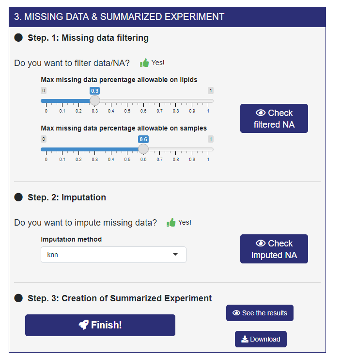
- Step 1. In the first step ADViSELipidomics computes the percentage of NAs, for each lipid (matrix rows) and each sample (matrix columns). Second, it allows retaining only lipids and/or samples with a percentage of missingness below thresholds chosen using the sliders. For example, if you set Max missing data percentage allowable on lipids to 0.3 Max missing data percentage allowable on samples to 0.6 that means that only lipids (rows) with less than 30% of NAs and samples (columns) with less than 60% of NAs are stored. After that, by clicking on the “Check filtered NAs” button, ADViSELipidomics provides the missing data distributions and the data dimension before and after filtering NAs.
- Step 2. Next, you can impute the remaining NAs with different imputation methods, three Not Model-Based (mean, median, and knn) and one Model-Based (irmi).
- Step 3. In the final step, ADViSELipidomics build the SummarizedExperiment object and download it. By clicking on the “See the results” you will be redirected to the next menu, SumExp Visualization.
4.3 SumExp Visualization
Once you ended successfully the Preprocessing module, the first thing that you can do is check the just created SummarizedExperiment (SE) object. This can be done in the SumExp Visualization menu. The complex structure of the SE object can be explored by a red gear icon where you can choose what part of the SE object should be shown and summarise the data (if you have technical replicates).
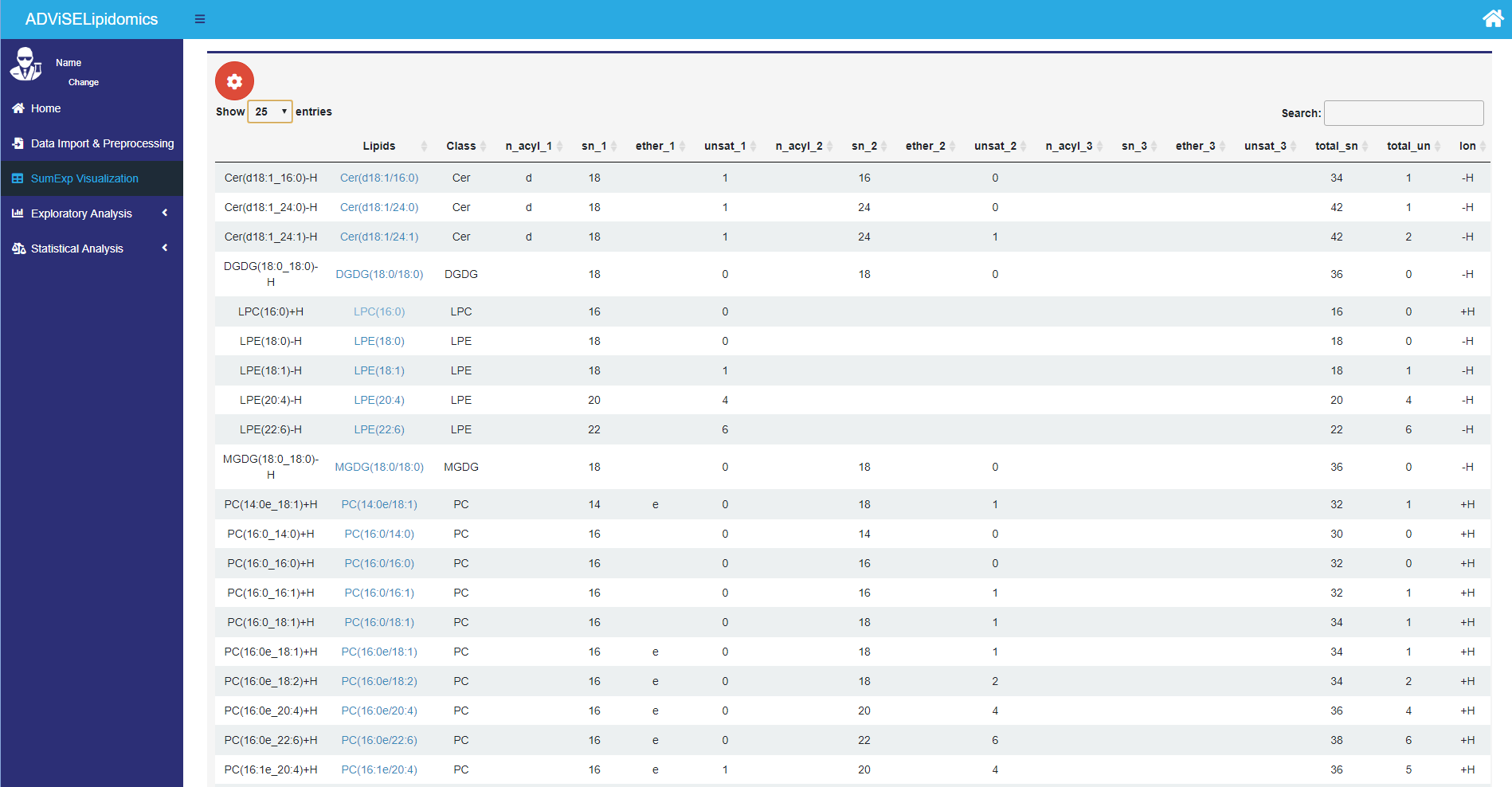
The picture above shows the rowData part of the SE object containing the annotation on lipids. Each lipid in the “Lipids” contains a hyperlink to the SwissLipids online repository to provide structural, biological, and analytic details.
4.4 Exploratory Analysis
The Exploratory Analysis menu includes three sub-menus: Plots, Clustering, and Dimensionality Reduction.
4.4.1 Plots
This sub-menu allows the user to create different types of plots to show the trend and behavior of data, exploring them from lipid and/or sample points of view. It has four panels: Lipids, Scatterplot, Heatmap, and Quality plots.
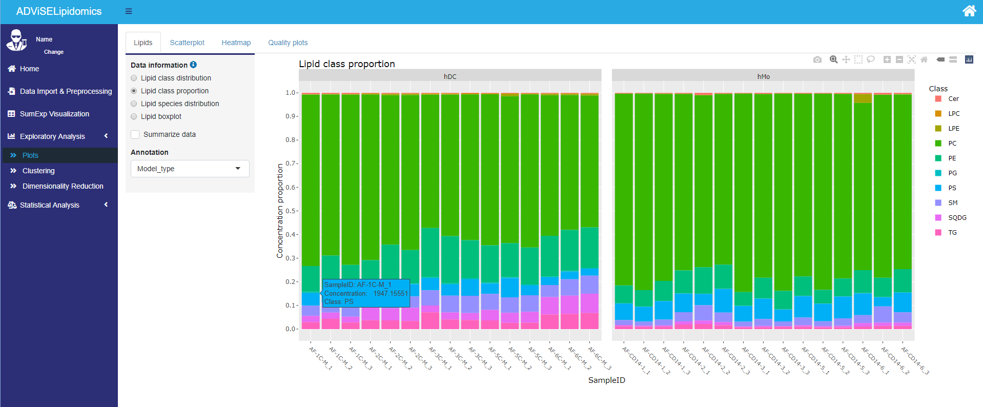
- Lipid plots. It is possible to 1) represent the lipid class distribution (counts of lipids per class) with a pie chart, boxplot, and spider plot; 2) visualize the percentage proportion of lipid class for each sample using a barplot, 3) compare the lipid species abundance for each condition; 4) inspect the abundance of a lipid, selected by the user, in relationship with a feature from the target file (e.g., treatment) using boxplots;
- Scatterplots. It is possible to visualize the relationship between lipid abundance in two samples;
- Heatmap. It provides a highly customizable heatmap to show possible clusters among lipids or samples. The user can select many parameters: a) row annotation with the feature from the target file, b) column annotation with the information from lipids parsing, c) dendrograms for lipids and/or samples, d) distance function (Euclidean, maximum, Canberra), e) clustering method (complete, average, median, Ward); f) number of clusters for lipids and/or samples. The user can select an area in the overall heatmap and have a detailed zoom of the area itself, with associated information;
- Quality plots. It provides different typologies of plots (barplot, boxplot, density plot) to show the total amount of abundance (logarithmic scale) per sample, considering as reference a feature from the target file, to show possible unexpected behavior among samples or replicates for the same sample.
The picture below shows an example of the Lipid class proportion plot.
4.4.2 Clustering
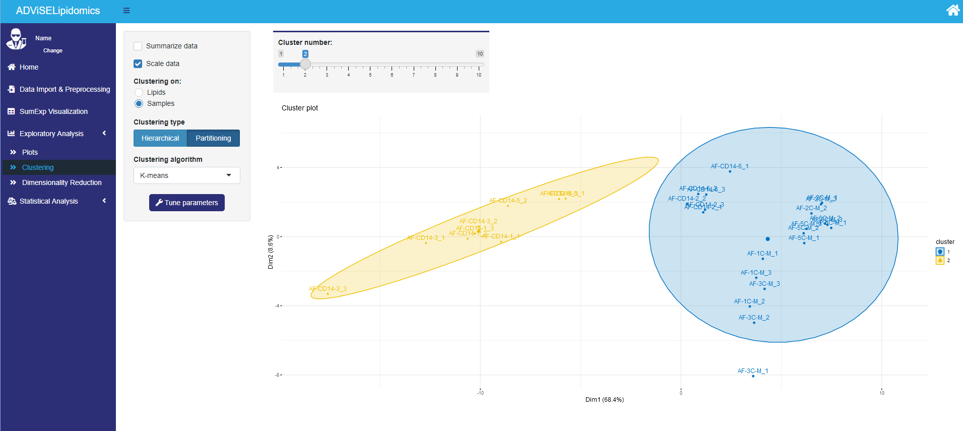
The Clustering sub-menu allows the user to cluster the data by lipids or samples. The user can choose the number of clusters and the clustering method among the following algorithms: hierarchical clustering (using single, complete, Ward as linkage function) or partitioning clustering (k-means, PAM, Clara). If you choose a partitioning clustering, ADViSELipidomics performs before a PCA. Additional plots, such as the silhouette plot, can suggest the number of clusters to use.
4.4.3 Dimensionality Reduction
The Dimensionality Reduction sub-menu allows the user to choose between unsupervised (PCA) and supervised approaches (PLS-DA, sPLS-DA) to represent the data in a two or three-dimensional space. It contains three panels PCA, PLS-DA, and sPLS-DA.
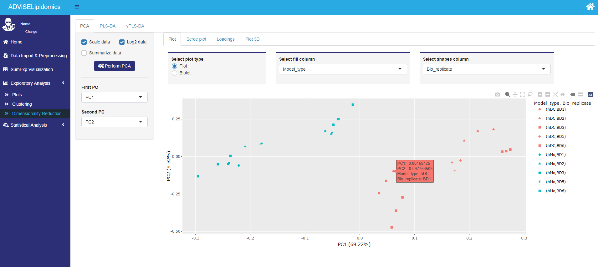
- PCA. ADViSELipidomics computes the Principal Component Analysis (PCA), showing the results with different plots: a) 2D plot, b) biplot, c) scree plot, d) loadings plot, e) 3D plot. The user can highlight the features from the target file with different colors and select the number of components to use for the loading plots.
- PLS-DA. ADViSELipidomics computes the Partial Least Square - Discriminant Analysis, showing the results with a 2D plot and a Correlation Circle plot. The user can select the group variable and the number of components for the computation. The 2D plot can be customized from the red gear icon. Furthermore, ADViSELipidomics can perform a Cross-Validation to identify the best number of components. It may take a while.
- sPLS-DA. ADViSELipidomics can compute also the sparse version of the PLS-DA. The panel is very similar to the PLS-DA panel, but since it’s a sparse version, it is possible to choose the number of variables to select on each component (called “KeepX”). Still here ADViSELipidomics can perform a Cross-Validation that helps the user to choose the best number of components and the best “KeepX”.
Here’s an example of a 2D plot for the PCA.
4.5 Statistical Analysis
The Statistical Analysis menu includes two sub-menus: Differential Analysis and Enrichment Analysis.
4.5.1 Differential Analysis
The Differential Analysis sub-menu applies statistical algorithms to identify lipids with a different abundance among samples associated with experimental conditions (i.e., treatment versus control). It has two panels: Build DA and Comparisons. The first allows the user to build and run the differential analysis, while the second shows the “differential expressed” lipids with a Venn Diagram and an Upset plot.
The picture below shows the first panel, Buil DA, with the different parts enlightened in red rectangles.
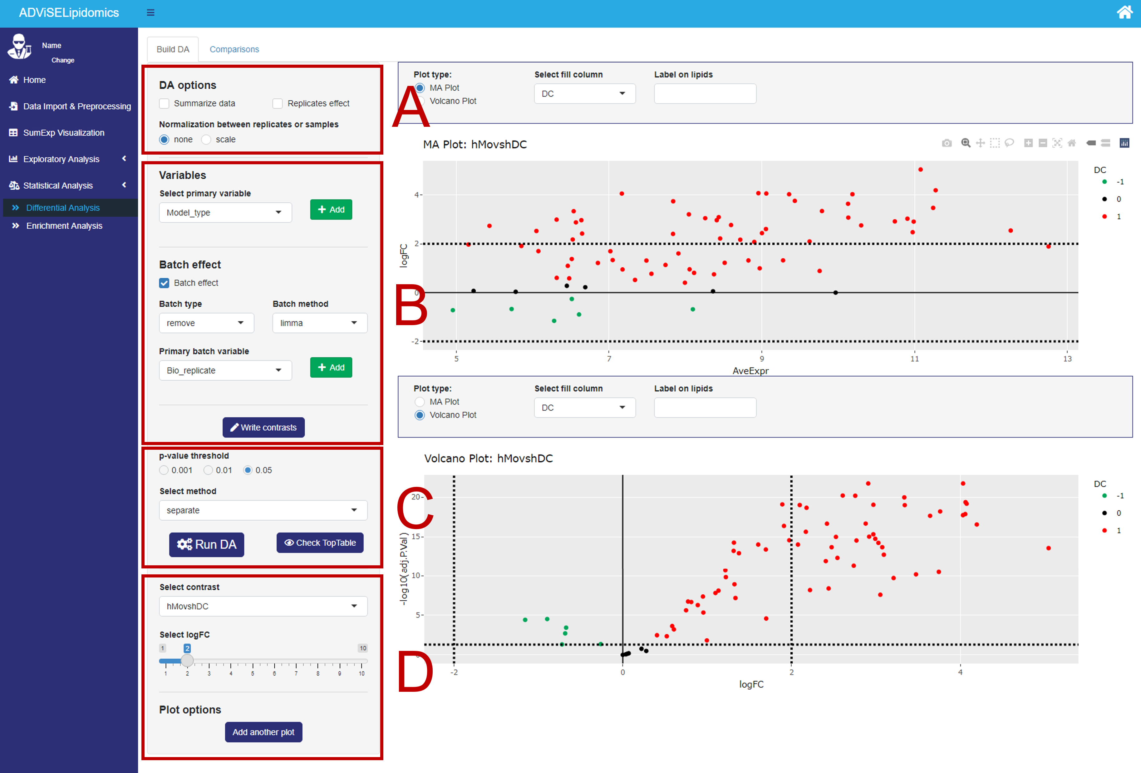
- Rectangle A. Here, you can select between one of the two SE objects obtained from the previous steps (i.e., the one with the lipid abundance of all samples or where the technical replicates are averaged). It is possible to normalize the data matrix by a scaling factor at this stage (“Normalization between replicates or samples”). Moreover, when a data matrix has technical replicates, you can even incorporate the replicate effect in the model by checking the “Replicates effect” box.
- Rectangle B. Here, you can build your experimental designs. An ADViSELipidomics complex design can include up to two experimental conditions and at most two variables to consider as batch effects. First, you can select a primary variable, and with the plus button, you can add a second variable. Next, you can decide to consider the batch effect by choosing up to two batch variables. More in detail, ADViSELipidomics copes with the batch effects by either fitting the model with the batch variables or removing the batch effect before fitting the model. To handle the batch effect, ADViSELipidomics uses the removeBatchEffect function from the limma package or the ComBat function (parametric or non-parametric method) from the SVA package. Finally, with the “Write contrasts” button, it opens a box where you can generate the contrast list. This functionality works with up to two total variables (e.g. primary variable + secondary variable (“Batch type” set to “remove”) or primary variable + primary batch variable with “Batch type” set to “fit”).
- Rectangle C. Here, you can select a threshold for the adjusted p-values, and a method for the decideTests function (limma package) used to identify “differentially expressed” lipids. Finally, click on the “Run DA” button to run the differential analysis. You can also check and download a table of results (TopTable).
- Rectangle D. In this rectangle there are some plot options, as the choice of the contrast, the threshold for the logFC, and the possibility of adding another plot. There are two different plots: a volcano plot and a MA plot, both interactive where you can change the fill variable and add labels to lipids of interest.
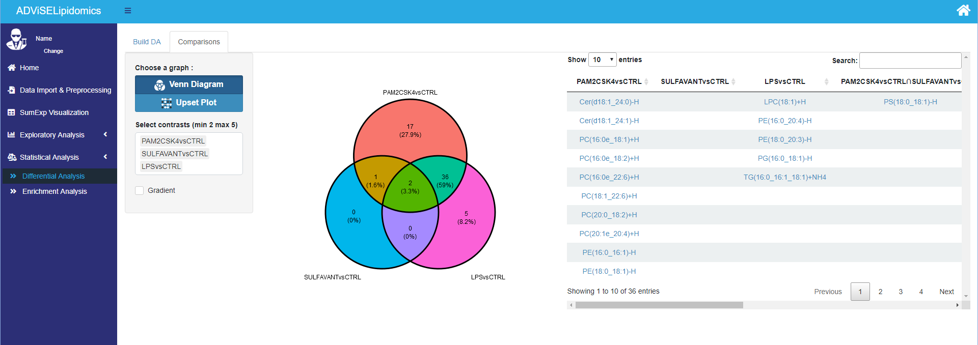
After ADViSELipidomics performed the DA, you can go to the Comparisons panel to visualize the “differential expressed” lipids and perform pairwise comparisons between different contrasts using the Venn diagram and the Upset plot. Finally, it reports the list of common lipids in tabular form. These two plots are available only with at least two contrasts.
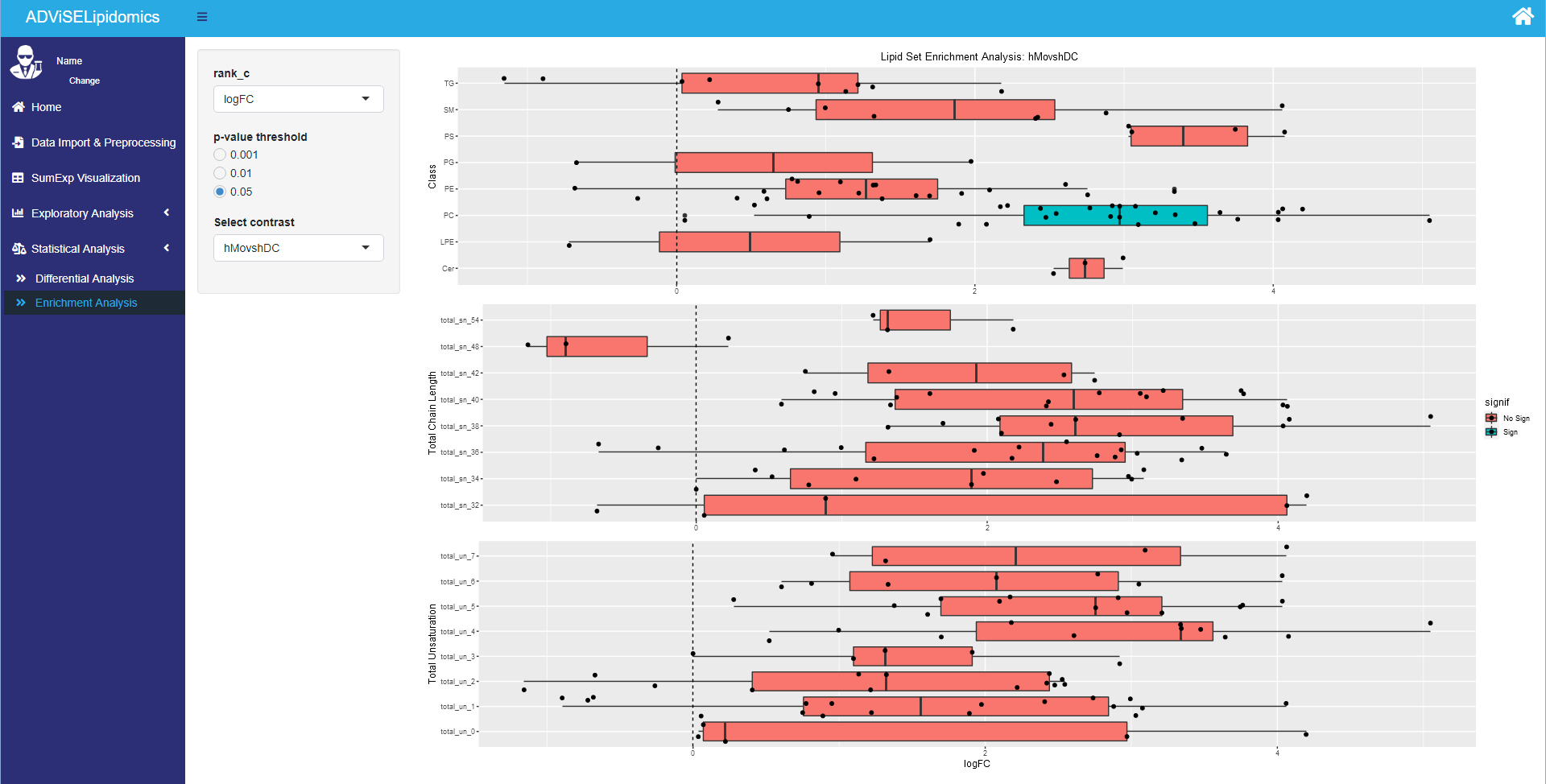
4.5.2 Enrichment Analysis
The Enrichment Analysis sub-menu allows for building different lipid sets from the chemical features of the lipids: i.e., lipid classes, total chain length (the sum of all carbon atoms in the tails), total unsaturation (the sum of all the double bonds in the tails). After defining a ranking for the differential abundant lipids (i.e., ranking considering logarithmic Fold Change, p-value, adjusted p-value, or B statistic), it identifies enriched sets of lipids using a permutation test. To achieve a robust result, it was necessary to perform a few million permutations, hence this process may take a while. Since Enrichment Analysis takes as input the differential analysis results, you need first to run the last one.